this recipe is still under construction!
What is Feature Engineering
Feature engineering means improving your data quality through transformations. This is extremely useful in improving the quality of your model. For instance, in the Kaggle Titanic competition, you can transform the text of a ticket number to infer the passenger class. Check out this excellent notebook with feature engineering techniques on the Titanic dataset and TDS article on many types of feature engineering (with examples!).
Feature engineering requires domain expertise and the ability to see past the immediate raw data to the story it could tell. Great feature engineering takes time, but provides you extra percentage points of accuracy. Bad feature engineering can result in misrepresenting your data and hurting your results.
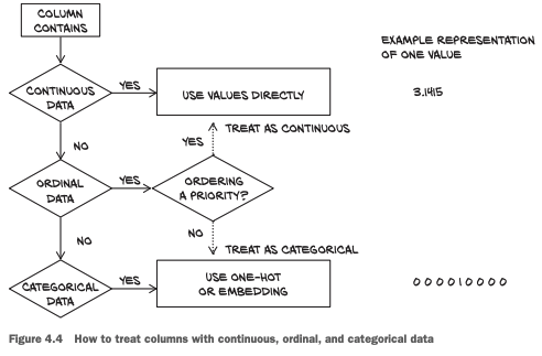
How to handle categorical and continuous features. Source
Imputation
Missing values within a dataset can cause errors when you run your code. To handle missing values, there are a few options. You can drop rows (instances) with missing values (e.g. if you are predicting house prices and a few homes don’t have a value for ‘total square feet’). You can also drop entire feature columns if most of the values are missing (e.g. if predicting house price and the ‘has a pool’ feature is mostly empty.
Common ways of filling in missing values are to use the mean or median value of a feature column. Be careful when imputing with the mean, because a long-tail distribution can move your mean and make it a poor value for imputation. Sometimes for categorical variables you can use the most-frequently occurring category. Here’s a longer explanation of different imputation approaches.
Handling Outliers
An outlier is a data point that is far from all your other data points. It could be naturally occurring (Jeff Bezos’ wealth in a dataset of American household wealth), a data transcribing error, or due to other reasons. Outliers can skew your data and cause violations in the assumptions of your models. But don’t have a blanket policy of dropping outliers, that’s not always the best policy.
You can find outliers by using standard deviation, Z-score, box plots, scatter plots, or percentile (often below 1st/5th percentile or above 95th/99th percentile). You can probably remove your outliers if one of the following is true:
- You have a few outliers among a lot of data
- The outliers will skew your data
- The outliers don’t reflect reality
You can also drop or cap outliers. Dropping removes them from the data set, but capping sets the outlier value to the “capped” value that falls better within the data distribution. For instance, if you thought Jeff Bezos would generally behave as someone in the 99th percentile of American household wealth (closer to $10M), then you could cap/set his wealth in your dataset at that 99th percentile value.
Binning
Binning can help normalize the distribution of the data. For instance, if you have some common and some rare values, grouping them together will even out the distribution of values. In the case of continuous variables, binning will also discretize them which may help make your results more interpretable as well. For instance, rather than representing people by their age, you may want to group them by age groups to avoid overfitting.
While there are no hard and fast rules on how to bin variables, some guidelines are as follows:
- If you’re trying to maximize interpretability, bin based on intuition–use subject matter expertise to select groupings that make sense (e.g. age by teen, young adults, middle age, seniors)
- If your priority is normalizing the data, bin based off of quantiles or a similar measurement such that each bin has similar number of data points.
- If you’re looking for something quick and easy, just use a fixed width (e.g. every 10 years, every 100 points on a PT test).
Encoding
When passing your categorical variables through an algorithm, you’ll have to encode them into numbers so that the model can understand that they are categories.
Label Encoding
The easiest way (and least memory intensive) is to conduct label encoding. That means you map each unique categorical value to a number. For instance, if your groups are baby, child, teen, adult, you could convert it to 0,1,2,3, respectively. This is perfect if there is a natural order in the categories (increasing/decreasing). However, if the categorical values are something like orange, apple, and blueberry; mapping them to 0,1,2, respectively is meaningless and may skew model results as blueberry will have more weight than apple for no good reason. On the other hand if the fact that blueberries are the most tasty fruit is of consequence, then using label encoding may make sense.
One Hot Encoding
One hot encoding is when you convert each category into a binary (0/1) value. When you categories do not have a natural order, this is likely the best way to represent the categories without misrepresenting the data. However, it is at the cost of adding a lot more variables to your data. A hundred different categories in a variable equates to a hundred more columns with values of 0 or 1.
Hashing
When you have many categories in a feature (called high cardinality), one hot encoding may not be practical. By hashing the features, you can take what would have been 100,000 new features, and encode it as 100 features. There may be collisions (different inputs being hashed into the same output), if you have a low dimensionality output, but this is fairly low risk and may not even have a huge impact on accuracy.
Feature Splitting
Sometimes one feature (especially strings values) may carry multiple nuggets of information. For example, if you have an “address” feature, you may want to split it into multiple features like street, city, state, and zip code.
Scaling
If you have multiple numerical features with wildly different ranges (e.g. physical training scores going up to 300 and number of years in the DoD up to 30), you should normalize them to all be in the same scale (e.g. 0 to 1). Otherwise your model will weight physical training scores heavier than the number of years in the DoD. In the case of regressions, this difference will likely be adjusted by the coefficient value, but may lead to misinterpretation of the importance of each feature if the coefficient of PT scores was significantly smaller than the coefficient for the number of years in the DoD.
Transformations
Transformations are primarily used in regression models where normality/linearity are key assumptions. They may be used to reduce skewness, stabilize variance, and/or normalize your data. Many of these techniques will come at a cost of reduced interpretability. When taking transformations of your data, you should plot the before and after to verify that the desired improvement was actually made. The following are a couple common techniques.
- Log Transform:
log(x). Often used to counter right-skew or positive skew (long right tail) in data. Your mileage may vary, don’t blindly do a log transformation. - Squareroot transform:
sqrt(x). Useful for when you have a huge range in values (e.g. number of bacteria in 1 cubic foot of soil vs number of earthworms) - Reciprocal:
1/xOnly works if you have nonzero values…will drastically alter the distribution of your data.
Feature Interaction
If you’re interested in how two features interact with each other, you may want to add an interaction term. They’re most commonly the product of two features, (e.g. feature_3 is feature_1 * feature_2) but can also be the sum or differences between features. It’s important to make sure the interaction terms and original features are not highly correlated.
Removing Non-Important Features
Multicollinearity
If you have instances of multicollinearity in your independent variables, you may drop one of them or wrap them up as an interaction term. Including both will cause redundancy at best, decreased impact to a predictor, and at worst overfitting. Pandas .corr() and seaborn’s heatmap can be used to visualize this.
Correlation
If an independent variable has a low correlation to the dependent variable, it may be better to just drop it. Keeping it may just add noise to your model and decrease accuracy overall.
Learn More
- 7 Feature Engineering Techniques (Analytics Vidhya)
- Feature engineering for NLP
- Feature engineering for Computer Vision
- More image augmentation techniques like flipping, adding noise, rotating, lightening/darkening, scaling, and more.
- Automated Feature Engineering (Towards Data Science)
- FeatureTools, an Automated Feature Engineering Library
Navigation
» Previous recipe
» Next recipe
» About
» Ingredients
» All recipes
» Resources
» Code examples